Insights
Technical notes and articles
Reproducible studies and analysis on observability, measurement and intelligence for distribution and transmission grids.
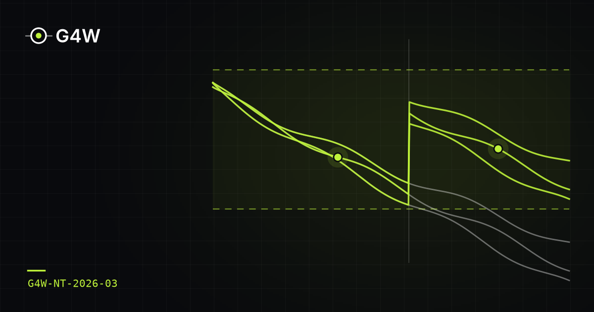
Voltage compensation payments that should already have stopped: what a few medium-voltage sensors change in diagnosis and in proving that the problem was fixed
When a 168-hour measurement finds voltage outside the limits, the Brazilian utility compensates the customer every month until a new measurement proves the problem has been fixed. Part of this payment is avoidable: it continues after a repair that has already solved the problem, or it repeats because the repair was done in the wrong place. This note quantifies what a few synchronized sensors on the medium-voltage network change in two decisions in the process: before the repair, telling whether the cause is on the medium- or low-voltage network; after the repair, telling whether the customer is back within limits. We simulated 13 types of problem (7 on medium voltage and 6 on low voltage) on the IEEE 34 test feeder with a modeled low-voltage network, 188 cases and 5,948 compensated customers, with a realistic network records model: unknown regulator positions and load, impedance and phase errors. For regulator problems, the estimator without sensors identifies the origin of the problem in 7% to 33% of cases, because it believes the regulator is working; with two sensors, it gets it right in 93% to 100%. After the repair, the errors about which customers are back within limits, which added up to 16%–48% of customers, drop to 4%–7%. For low-voltage problems, the sensors help rule out medium voltage as the cause (accuracy rises from 80–87% to 93–100%), but they cannot tell whether the customer is back within limits: that requires measuring at the customer. In two types of problem, the model is so far from the real network that the estimator fails to converge 35% to 60% of the time.
Why doesn't the state estimator converge? Load data quality, automatic cleaning and the role of a few sensors
In distribution networks, the state estimator relies on load pseudo-measurements built from customer meters and typical load profiles, with incomplete coverage, different integration intervals, missing data, and customers with their own generation whose meters do not report the direction of power flow. Using three three-phase test feeders (IEEE 13, 34 and 123 bus) with photovoltaic generation at 30% of the loads, this note quantifies the effect of these defects on a nonlinear weighted least squares estimator and compares three approaches: using the data as received, cleaning it before estimation, and applying automatic cleaning based on normalized residuals. With raw data, 30% to 53% of the estimates are rejected by the consistency test, and the voltage error reaches 10% in one out of ten scenarios on IEEE 34. Prior data treatment lowers the rejection rate to 0.5%–6% and reduces the median voltage error by 27% to 50%. Automatic cleaning without network measurements masks the problem: rejection drops but the error does not, and on IEEE 34 the estimator fails to converge in 12% of cases. With two to four synchronized sensors, the same cleaning starts to work on the smaller feeders, and treated data with four sensors brings the median voltage error down to 0.10%–0.20%. The individual load at each bus remains dependent on the quality of customer data.
How many sensors, and where? Synchronized measurement placement for three-phase state estimation in distribution feeders
Many distribution feeders are only metered at the substation, and state estimation along the network relies on load forecasts with high uncertainty. Using three unbalanced three-phase test feeders (IEEE 13, 34 and 123 bus), this note shows how much the estimation error drops when synchronized measurement points are added to the network, how much the choice of those points matters, and what measurement and timing accuracy that gain requires. With four points, chosen by a greedy procedure and evaluated on independent scenarios, the average of the largest voltage error per scenario drops by 90%, 94% and 59%, and the line-section current error drops by 89%, 82% and 44%. If the substation only provides typical SCADA quantities (current magnitude and power), the case without points gets worse and the reduction rises to 91%, 94% and 65%. Optimized placement brings the voltage error below 0.3% with two to four points, while a uniform spacing rule needs five or never gets there, and the average random placement does not get there with eight points on two feeders. Timing with a standard deviation of up to 10 µs preserves at least 98% of the gain. The individual load at each bus improves much less when there are many loads per point.