How many sensors, and where? Synchronized measurement placement for three-phase state estimation in distribution feeders

1. Introduction

Distributed generation, electrified loads and bidirectional flows make the voltage profile and loading of a feeder less predictable than in a network with only passive loads. Even so, many feeders are instrumented only at the substation. Between the substation and the end of the network there can be kilometers of conductor with no measurement at all.

State estimation combines sparse measurements with a network model to produce a complete picture: voltages at every node and, from them, line-section currents, loads and losses [1], [2]. In distribution, the lack of measurements forces the estimator to use pseudo-measurements, that is, consumption forecasts derived from billing or typical load profiles, with high uncertainty [3]. On top of that, phase unbalance requires three-phase modeling.

Synchronized sensors measure voltage and current magnitude and angle at points distributed across the network, with a common time reference, typically obtained from GNSS [4], [5], [11]. For a utility, the practical question is not whether these sensors help, but how many points to instrument, where, and with what measurement and timing accuracy, because each point carries equipment, installation and communication costs. Measurement placement has been studied for decades in transmission [6].

This note is an open and reproducible study of these decisions, prepared by G4W to show how we evaluate an instrumentation design. The estimator (weighted least squares) and the placement method (a greedy procedure) were chosen because they are simple, transparent and easy to reproduce with the published code. They do not describe the algorithms in G4W products, nor do they claim to be the best available method. The goal is to show, on public cases, how instrumentation design choices change the outcome.

2. Formulation

2.1 State and measurements

Consider the three-phase network with $n$ nodes (each phase of a bus is a node) and nodal admittance matrix $\mathbf{Y}$. The matrix includes lines, transformers, regulators at their current tap, capacitors and the source equivalent, but not the loads. The state is the vector of complex nodal voltages $\mathbf{x} = [V_1, \dots, V_n]^\top$.

The vector $\mathbf{Y}\mathbf{x}$ gives the current injected into the network at each node by the elements that are not in $\mathbf{Y}$. At a load node, $-(\mathbf{Y}\mathbf{x})_k$ is the current drawn by the load. At a node with no load and away from the source, this injection is zero.

Why the main estimator is linear. The relation $\mathbf{I} = \mathbf{Y}\mathbf{V}$ is linear in the complex state. Power, $S = V\,\overline{I}$, is not. In the conventional formulation, where forecasts enter as powers, the estimator is nonlinear and solved iteratively. Here, all quantities used in the main estimator are voltage or current phasors (measured, forecast or zero), so the measurement model is linear:

$$\mathbf{z} = \mathbf{H}\,\mathbf{x} + \mathbf{e},$$

where $\mathbf{e}$ collects the measurement and forecast errors. The estimator weights use a matrix $\mathbf{R}$ that approximates the covariance of these errors; the points where it departs from the simulated error are listed in Section 5. Table 1 summarizes the measurements.

Type	Where	Quantity (per phase)	Assumed standard deviation
Substation measurement	source bus, substation bus and feeder head section	voltage phasors; feeder head current (phasor or, in the SCADA variant, current magnitude and powers)	0.1% (voltage); 0.5% (current); 1% (powers in the SCADA variant)
Synchronized measurement point	start of a line section	voltage phasor at the sending bus; phasor of the current entering the section	0.2% and 0.5% in magnitude, plus the timing error
Pseudo-measurement (forecast)	load nodes	forecast load current	50% of the forecast current magnitude of each load branch
Zero injection	nodes without load	$(\mathbf{Y}\mathbf{x})_k = 0$	minimum variance (very high weight)

Pseudo-measurements. A pseudo-measurement is not a measurement: it is the load forecast, which the utility knows before measuring any point on the network. For a load with forecast power $\tilde S$ connected between nodes $a$ and $b$ (node $b$ is ground for wye-connected loads and another phase for delta-connected loads), the forecast current is

$$\tilde I_{ab} = \overline{\left(\frac{\tilde S}{V^{0}_a - V^{0}_b}\right)},$$

where $V^{0}$ are the no-load network voltages, with the base case taps. For three-phase loads, the forecast power is split equally between phases. Using a fixed voltage $V^0$ is what keeps the model linear. The cost is an approximation: the actual current depends on the actual voltage at that point and on the load model (constant power, current or impedance). This difference adds to the forecast error and can introduce small biases not represented in $\mathbf{R}$.

A delta load injects $-\tilde I_{ab}$ at node $a$ and $+\tilde I_{ab}$ at node $b$, so the pseudo-measurements at those nodes are correlated. That is why the pseudo-measurement block of $\mathbf{R}$ is full: $\mathbf{R}_{\text{pseudo}} = \mathbf{A}\,\boldsymbol{\Sigma}\,\mathbf{A}^{H}$, where $\mathbf{A}$ maps load-branch currents to nodes and $\boldsymbol{\Sigma}$ is diagonal. Nodes without load enter the same block with a minimum variance, which amounts to a very high weight rather than an exactly enforced equality.

Measurement points and timing. Each point sits at the start of a line section and measures, per phase, the voltage at the sending bus and the current entering the section, $\mathbf{I} = \mathbf{Y}^{\text{prim}}_{1,:}\,[\mathbf{V}_1;\,\mathbf{V}_2]$. Magnitude errors are Gaussian and relative. The angle error comes from timing: a time error $\delta t$ produces, at 60 Hz,

$$\delta\theta = 2\pi f\,\delta t \approx 0.0216^\circ \text{ per microsecond}.$$

In each scenario, the time error of each point is drawn with standard deviation $\sigma_t$ relative to the substation reference, independently across points, and the same angle is applied to that point's voltage and current. Thus $\sigma_t$ is not the maximum error between pairs (the difference between two points has standard deviation $\sqrt{2}\,\sigma_t$), does not include other angular errors in the measurement chain (instrument transformers, filtering, phasor estimation), and has nothing to do with communication latency.

2.2 What K = 0 means

In this text, $K$ is the number of additional measurement points on the network, beyond the substation. A point is the start of a line section where all phases present are measured; the number of physical devices per point depends on the technology (with sensors installed on the conductor, a three-phase point may need one device per phase). The results count points, not devices.

K = 0 means zero additional points, not an absence of information. The estimator has the substation measurement, the load forecasts and the zero injections. The injection equations at all nodes (forecast or zero), together with the voltage measured at the source, already form a system equivalent to a linear power flow: given the source voltage and the current at each node, the voltages are determined. On the three feeders studied, this system has full rank and the solution is unique. The network is therefore observable thanks to the forecasts, not only through physical measurement.

The only redundancy comes from the substation. In practice, the estimator does an allocation: it forces the total current of each phase to match the feeder head measurement and distributes the difference between measured and forecast among the loads, according to the uncertainty assigned to each. A variation common to all loads (time of day) is corrected well. An individual variation is not, because the estimator has no way of knowing in which branch it occurred. This is the case against which we measure the gain from additional points.

2.3 Estimator

The weighted least squares estimate is

$$\hat{\mathbf{x}} = \left(\mathbf{H}^{H}\mathbf{R}^{-1}\mathbf{H}\right)^{-1}\mathbf{H}^{H}\mathbf{R}^{-1}\,\mathbf{z},$$

computed by QR decomposition of the weighted system, with columns scaled by each node's base voltage (the admittances of switches and regulators differ by several orders of magnitude from those of long line sections, which would make the normal equations ill-conditioned). From $\hat{\mathbf{x}}$ we obtain the line-section currents, $\hat{\mathbf{I}} = \mathbf{Y}^{\text{prim}}\hat{\mathbf{V}}$, and the load at each bus, $\hat S_b = \sum_{k \in b} \hat V_k\,\overline{\big(-(\mathbf{Y}\hat{\mathbf{x}})_k\big)}$, computed after estimation.

In the SCADA variant (Section 4.3), the feeder head is measured as current magnitude per phase and three-phase active and reactive power. These measurements are nonlinear in the state, and the estimate is obtained by Gauss-Newton in rectangular coordinates, starting from the linear solution without the feeder head measurement.

The estimator is not the power flow. The "ground truth" for each scenario comes from the OpenDSS power flow, which solves the nonlinear network equations with the original load models. The estimator only combines measurements and forecasts with a fixed $\mathbf{Y}$.

The standard deviations of measured currents are proportional to the current magnitude. To size them, we use the currents from a power flow with the forecast loads, information available before any measurement.

Check. With exact measurement on every line section, the estimator recovers the OpenDSS solution with a voltage error below $10^{-4}\,\%$ on all three feeders, also in the SCADA variant, and the matrix $\mathbf{Y}$ reproduces the power flow injections with a residual below $10^{-5}$ A at nodes without load.

2.4 Metrics

For each of the $N$ evaluation scenarios, three errors are computed, and the results are averages over the scenarios.

Voltage — the largest magnitude error among all nodes (except the source nodes), in % of the node's base voltage:

$$\varepsilon_V = \frac{1}{N}\sum_{s=1}^{N}\ \max_{k}\ \frac{\big|\,|\hat V_{k,s}| - |V_{k,s}|\,\big|}{V^{\text{base}}_k}\times 100\,\%.$$

This is an average of per-scenario maxima, not a worst-case bound; where useful, we also report the 90th percentile.

Current — for each line section, the largest magnitude error among the phases, summed over the sections and divided by the sum of each section's largest true current:

$$\varepsilon_I = \frac{1}{N}\sum_{s}\frac{\sum_\ell \max_{p}\big|\,|\hat I_{\ell p,s}| - |I_{\ell p,s}|\,\big|}{\sum_\ell \max_p |I_{\ell p,s}|}\times 100\,\%.$$

Load — sum of the active power errors per load bus, divided by the total load:

$$\varepsilon_P = \frac{1}{N}\sum_{s}\frac{\sum_b |\hat P_{b,s} - P_{b,s}|}{\sum_b |P_{b,s}|}\times 100\,\%.$$

On IEEE 123, bus 610 (secondary of a delta transformer, with no load and no ground connection) is excluded from the voltage metric: there, the phase-to-neutral voltage has no physical meaning.

2.5 Placement

Given a budget of $K$ points, we look for the set $\mathcal{S}$ of line sections that minimizes

$$J(\mathcal{S}) = \frac{\varepsilon_V(\mathcal{S})}{\varepsilon_V(\varnothing)} + \frac{\varepsilon_I(\mathcal{S})}{\varepsilon_I(\varnothing)} + \frac{\varepsilon_P(\mathcal{S})}{\varepsilon_P(\varnothing)},$$

that is, the three errors, each relative to the $K = 0$ case, with equal weight. The problem is combinatorial (on IEEE 123, for $K = 4$ among 123 sections, there are about 9.1 million combinations). We use a greedy procedure, common in sensor placement [7]: at each step, the section that most reduces $J$, estimated on the selection scenarios, is added, without revisiting earlier choices. The set for each $K$ is the beginning of that sequence.

The greedy method does not guarantee the optimum. To check it, we ran an exhaustive search where it was feasible. On IEEE 13, the greedy method found exactly the best set for $K = 1$ to 4. On IEEE 34, it found the best set for $K = 1$ and 2; for $K = 3$ and 4, the best set is different, but its objective is less than 1% lower, a difference on the order of the Monte Carlo variation. On IEEE 123, the check was only feasible for $K = 1$, where both coincide.

3. Case study

We used three IEEE test feeders [8], from the public OpenDSS files [9], [10]: three-phase and unbalanced, with single- and two-phase laterals, wye and delta loads, and voltage regulators (Table 2).

Feeder	Voltage	Total load	Load buses	Nodes	Regulators (phases)	Candidate sections
IEEE 13	4.16 kV	3.47 MW	9	41	3	11
IEEE 34	24.9 kV	1.77 MW	28	95	6	31
IEEE 123	4.16 kV	3.49 MW	85	278	7	123

Scenarios. The ground truth for each scenario is the OpenDSS power flow, with the original load models, after perturbing the loads around the forecast by a factor common to all (15% standard deviation, time of day) and an individual factor per load (30%), both truncated. Regulator taps are those of the base case, held fixed. The points are chosen with 120 scenarios and evaluated on 400 other, independent ones.

Strategies compared, all evaluated on the same 400 scenarios:

1. Optimized (greedy), described in Section 2.5.
2. Uniform along the main trunk, a simple reference rule: the $K$ points are spaced equally, by number of sections, along the path between the source and the most distant bus. On IEEE 13 the trunk has only four sections, so the rule uses at most four distinct points.
3. Random: 30 random draws of sections for each $K$.

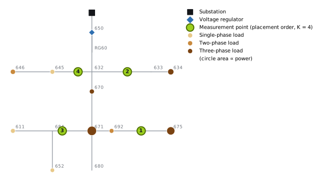
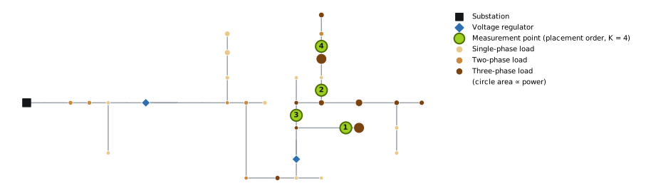
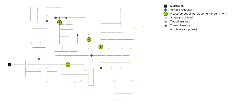
Figures 1 to 3 show the feeders, the loads (area proportional to power and color by number of phases) and the first four points of the optimized placement.

4. Results

In Sections 4.1, 4.2, 4.4 and 4.5, the feeder head is measured as a current phasor. This assumption favors the case without points; Section 4.3 shows what changes with typical SCADA quantities.

4.1 Error as a function of the number of points

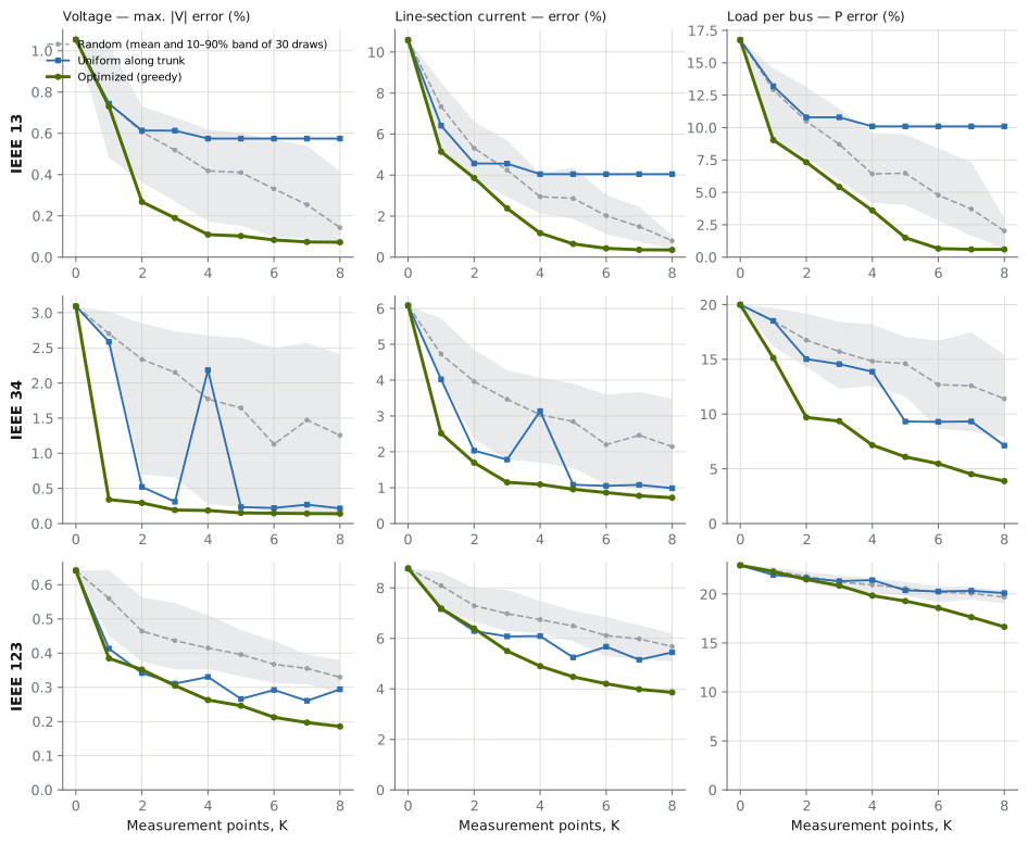
Figure 4 shows the three errors for $K$ from 0 to 8. Table 3 summarizes the voltage error.

Feeder	Strategy	K = 0	K = 1	K = 2	K = 4	K = 8
IEEE 13	Optimized	1.05%	0.73%	0.27%	0.11%	0.07%
	Uniform along trunk	1.05%	0.74%	0.61%	0.57%	0.57%*
	Random (mean)	1.05%	0.75%	0.61%	0.42%	0.14%
IEEE 34	Optimized	3.09%	0.34%	0.29%	0.19%	0.14%
	Uniform along trunk	3.09%	2.59%	0.52%	2.18%	0.22%
	Random (mean)	3.09%	2.70%	2.33%	1.77%	1.26%
IEEE 123	Optimized	0.64%	0.38%	0.35%	0.26%	0.19%
	Uniform along trunk	0.64%	0.41%	0.34%	0.33%	0.29%
	Random (mean)	0.64%	0.56%	0.46%	0.42%	0.33%

* With four distinct points, the most the IEEE 13 trunk can hold. The values are $\varepsilon_V$, the average over scenarios of the largest voltage error in each scenario. With the optimized placement and four points, the 90th percentile of this error is 0.16%, 0.30% and 0.36%, against 1.69%, 5.92% and 0.98% without points.

The first well-placed point can be worth a lot. On IEEE 34, the error without points is concentrated in the 4.16 kV lateral fed by the transformer between buses 832 and 888, which serves a 450 kW load at bus 890 (average error of 2.7% at that bus, against less than 0.5% in the rest of the network). A single point at the start of that lateral (section 888–890) reduces the error to 0.34%.

The choice of points matters as much as the number. To bring the voltage error to 0.3% or less:

• the optimized placement needs two points on IEEE 13, two on IEEE 34 and four on IEEE 123;
• the uniform rule needs five on IEEE 34 and five on IEEE 123, and never gets there on IEEE 13, whose trunk leaves out the laterals where the error is concentrated;
• the average random placement does not get there with eight points on IEEE 34 and IEEE 123; on IEEE 13, it gets there with seven.

The uniform rule is also unstable: on IEEE 34, going from three to four points shifts the positions along the trunk, removes the point from the critical lateral, and the error rises from 0.31% to 2.18%.

The number of buses does not determine the voltage error. IEEE 123, the largest of the three, has the smallest error without points (0.64%) and the smallest relative reduction with four points. The error depends on impedances, voltage level, loading, load location and regulator action; this study does not isolate the contribution of each factor.

Current and load respond differently from voltage. With four points, the line-section current error drops from 10.6% to 1.2% on IEEE 13, from 6.1% to 1.1% on IEEE 34 and from 8.8% to 4.9% on IEEE 123 (reductions of 89%, 82% and 44%, against 90%, 94% and 59% for voltage). The per-bus load error drops much less where there are many loads:

Feeder	Load buses	K = 0	K = 4	K = 8
IEEE 13	9	16.8%	3.6%	0.6%
IEEE 34	28	20.0%	7.2%	3.9%
IEEE 123	85	22.9%	19.8%	16.6%

A few well-placed points greatly improve voltages and flows, but when there are many loads downstream of each point, they are not enough to separate individual loads. With three feeders, this relationship is an indication, not a rule.

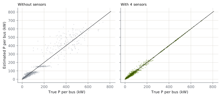
Figure 5 illustrates the effect on load for IEEE 34. Without points, the estimated loads vary little from one scenario to another (the horizontal bands): the estimator corrects the total using the current measured at the substation, but does not know which load changed. With four points, the estimates line up with the true load.

4.2 Where to install

For the most part, the chosen points are at the start of laterals or branches that feed relevant loads, not at the end of laterals or at equally spaced positions.

• IEEE 13: sections 692–675 (which feeds the largest three-phase load), 632–633 (which feeds the 480 V transformer), 671–684 and 632–645, on the side laterals.
• IEEE 34: the 4.16 kV lateral (888–890) and the branches 834–842, 832–858 and 844–846.
• IEEE 123: the trunk section 53–54, the branch 44–47, the switch between 97 and 197, and section 63–64. Here the pattern is less clear.

An intuitive reading, not tested in isolation: the current measured at the start of a lateral splits the load uncertainty between what is upstream and downstream of the point, and the zero injections carry that information along the lateral. A point at the end of a lateral measures only the last load; a point in the middle of the trunk measures the sum of many loads. Indeed, installing the points at the ends of laterals, from the farthest to the nearest, was much worse: with four points, 0.67% on IEEE 13, 2.70% on IEEE 34 and 0.41% on IEEE 123.

4.3 The substation measurement: phasor or SCADA

The results above treat the feeder head as a current phasor, synchronized with the substation reference. Many substations, however, deliver the current magnitude and powers to the control center. Figure 6 repeats the optimized placement with the feeder head measured this way.

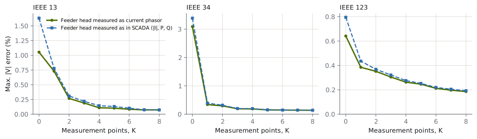
Voltage error	Phasor, K = 0	SCADA, K = 0	Phasor, K = 4	SCADA, K = 4	Reduction with 4 points (SCADA)
IEEE 13	1.05%	1.63%	0.11%	0.14%	91%
IEEE 34	3.09%	3.39%	0.19%	0.20%	94%
IEEE 123	0.64%	0.80%	0.26%	0.28%	65%

With SCADA measurement, the case without points gets worse (current magnitude and total three-phase powers do not determine the current angle in each phase), but with two or more points the difference practically disappears. Current and load errors barely change. To reach 0.3% voltage error, the optimized placement now needs three points on IEEE 13 and IEEE 34 and still four on IEEE 123. In other words, the reductions in Section 4.1 are a conservative estimate of the gain at a substation with conventional SCADA.

4.4 What the point should measure

Figure 7 keeps the four points of the optimized placement and varies the error of the point's voltage measurement, comparing it with a point that measures current only. The substation voltage reference, with 0.1% error, is still present.

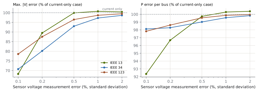
In this study, current accounts for most of the gain. Also measuring voltage reduces the estimated voltage error by 21% to 32% with a 0.1% measurement error, and by 10% to 20% with 0.2%. At 0.5%, the gain is already below 7%, and at 1% or more it practically disappears. For load estimation, the effect is small (up to 8% on IEEE 13 with 0.1%).

These numbers hold under the study's conditions: a 0.1% reference at the substation, fixed placement and a known network model. The literature on phasor-based estimation also shows that the value of each measurement depends on the quantity and accuracy of the whole set [12]; the range found here is not a general threshold. Nor is this an argument for dropping voltage measurement: voltage compliance, power quality, fault location and topology identification may justify it for reasons this note does not evaluate.

4.5 The role of timing

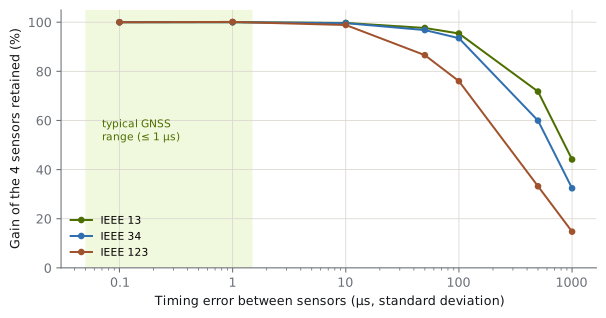
Figure 8 keeps the four points and varies $\sigma_t$, showing the fraction of the voltage gain (relative to $K = 0$) that is retained.

$\sigma_t$	IEEE 13	IEEE 34	IEEE 123
up to 10 µs	≥ 98%	≥ 98%	≥ 98%
100 µs	95%	94%	76%
1 ms	44%	32%	15%

IEEE 123 was the most sensitive; the study did not isolate the cause. The estimator knows $\sigma_t$ (the angular variance enters $\mathbf{R}$), but $\mathbf{R}$ does not include the correlation between the voltage and current errors of the same point. For reference, a field-deployed micro-synchrophasor network reported time alignment better than 1 µs between device pairs and angular accuracy of 0.01° [11], within the favorable range of this study. That metric (between pairs) is not identical to the one used here, and that result does not establish the cost or feasibility of a conductor-mounted sensor.

5. Discussion and limitations

On all three feeders, estimation quality was largely a matter of instrumentation design. The number of points needed depended on the topology, on the quantity to be estimated and on measurement and timing quality, and the choice of points mattered as much as their number. For anyone planning a monitoring program, the results suggest four guidelines, valid in these cases and to be confirmed on each network:

• Choose the points using the network model, not a spacing rule: the start of laterals that feed relevant loads was the most frequent pattern.
• A few points already change the quality of voltages and currents: two to four points brought the voltage error to 0.3% or less.
• Timing on the order of microseconds preserves practically all of the gain; errors on the order of milliseconds destroy it.
• To know the load at each bus, with many loads per lateral, network points need to be combined with other sources, such as customer smart metering.

The study has limitations:

• Known taps and model. The matrix $\mathbf{Y}$ uses the current taps and exact parameters. With an unknown tap, it should enter as a state variable; parameter errors were not addressed.
• Forecast model. The pseudo-measurement block of $\mathbf{R}$ treats each load branch as independent, does not represent the common factor or the joint variation of a load's phases, and uses a 50% variance, larger than the spread used to generate the scenarios. Converting power to current with $V^0$ is another approximation. Real loads have correlations, asymmetries and distributed generation; these differences may change the results, in a direction this study cannot determine.
• Approximate covariances. Zero injections enter with a high weight, not as an exact equality (lowering that floor did not change the results; raising it a hundredfold worsened the four-point IEEE 13 case from 0.11% to 0.14%). The correlation between the voltage and current errors of the same point, which share the clock, is not in $\mathbf{R}$.
• Snapshot in time and measurements without gross errors. Time series, communication loss and bad data detection were not addressed.
• Greedy placement. The exhaustive check was only possible in some of the cases, and the equal weighting of the three errors in the objective is a choice. Applications such as fault location would lead to different placements.
• Cost and physical implementation. Sensor cost, installation, power supply and communication were not evaluated.
• Generalization. Three test feeders do not allow extrapolating point-to-load ratios, or accuracy and timing thresholds, to real networks.

6. Conclusion

On three unbalanced three-phase test feeders, four synchronized measurement points, added to the substation measurement and chosen by a greedy procedure, reduced the average of the largest voltage error per scenario by 90% (IEEE 13), 94% (IEEE 34) and 59% (IEEE 123), and the line-section current error by 89%, 82% and 44%, evaluated on independent scenarios. With a substation that only provides SCADA quantities, the voltage reduction rises to 91%, 94% and 65%. The optimized placement, verified by exhaustive search where feasible, reached 0.3% voltage error with two to four points; a uniform spacing rule needed five or never got there. The gain depends on timing on the order of microseconds, and the individual load at each bus improves little when there are many loads per point. The practical message is that instrumentation design, and not just the number of sensors, determines much of the return on a network monitoring program.

Reproducibility

Code: se3f.py (network model, linear and SCADA estimators, metrics), study.py (placement, comparisons, exhaustive search, SCADA variant, voltage accuracy and timing) and figs_paper.py. Results: IEEE 13, IEEE 34, IEEE 123. Dependencies: Python 3.12 or later, OpenDSSDirect.py, NumPy and Matplotlib. The feeders are the IEEETestCases files from the public OpenDSS test case repository [10]. Main seed: 2026; the code fixes auxiliary seeds for measurement noise and random draws.

References

1. A. Abur and A. Gómez Expósito, Power System State Estimation: Theory and Implementation. New York: Marcel Dekker, 2004.
2. M. E. Baran and A. W. Kelley, "State estimation for real-time monitoring of distribution systems," IEEE Transactions on Power Systems, vol. 9, no. 3, 1994.
3. A. Primadianto and C.-N. Lu, "A review on distribution system state estimation," IEEE Transactions on Power Systems, 2017.
4. A. von Meier, E. Stewart, A. McEachern, M. Andersen and L. Mehrmanesh, "Precision micro-synchrophasors for distribution systems: A summary of applications," IEEE Transactions on Smart Grid, vol. 8, no. 6, 2017. doi: 10.1109/TSG.2017.2720543.
5. IEEE Std C37.118.1-2011, IEEE Standard for Synchrophasor Measurements for Power Systems, 2011.
6. T. L. Baldwin, L. Mili, M. B. Boisen and R. Adapa, "Power system observability with minimal phasor measurement placement," IEEE Transactions on Power Systems, vol. 8, no. 2, 1993.
7. A. Krause, A. Singh and C. Guestrin, "Near-optimal sensor placements in Gaussian processes: Theory, efficient algorithms and empirical studies," Journal of Machine Learning Research, vol. 9, 2008.
8. W. H. Kersting, "Radial distribution test feeders," in Proc. IEEE PES Winter Meeting, 2001.
9. EPRI, OpenDSS — Open Distribution System Simulator. Available at: https://sourceforge.net/projects/electricdss/
10. DSS-Extensions, OpenDSSDirect.py and electricdss-tst (OpenDSS test cases). Available at: https://github.com/dss-extensions
11. A. L. Liao, E. M. Stewart and E. C. Kara, "Micro-Synchrophasor Data for Diagnosis of Transmission and Distribution Level Events," Lawrence Berkeley National Laboratory, LBNL-1005925, 2016. Available at: https://eta-publications.lbl.gov/sites/default/files/lbnl-1005925.pdf
12. C. Muscas, M. Pau, P. A. Pegoraro and S. Sulis, "Uncertainty of Voltage Profile in PMU-Based Distribution System State Estimation," IEEE Transactions on Instrumentation and Measurement, vol. 65, no. 5, pp. 988–998, 2016. doi: 10.1109/TIM.2015.2494619.