Why doesn't the state estimator converge? Load data quality, automatic cleaning and the role of a few sensors

1. Introduction

Advanced distribution management systems (ADMS) use a state estimator to compute voltages, currents and loading across the whole network. In distribution, however, there is almost no measurement along the feeders. The estimator relies on load pseudo-measurements built from customer meters, measurement campaigns and typical load profiles per consumer class [1], [2].

This data arrives with problems well known to anyone who operates an ADMS: not every customer has a meter; those that do record at different intervals (5, 15 or 60 minutes); some intervals are missing; and for customers with their own generation, the meter often reports only the net value, or only the magnitude of the power, without the direction of flow. Add to this gross errors, such as 15-minute energy read as power. The visible symptom is an estimator that "doesn't converge": it either fails to converge or converges to a result the consistency tests reject, and the operator loses confidence in the tool.

This note answers three questions, with reproducible results on public test feeders:

1. How much does each way of handling load data change the reliability and the error of the estimator?
2. Can automatic cleaning, which discards suspicious pseudo-measurements based on the residuals themselves, replace prior data treatment?
3. How much do a few synchronized sensors installed on the network help, at the same locations chosen in the previous note in this series [3]?

2. Formulation

2.1 Estimator

The state is the vector of complex nodal voltages of the three-phase network, in rectangular coordinates and per unit of each node's base voltage. The measurements follow the pattern of an ADMS:

Measurement	Where	Model $h(\mathbf{x})$	Uncertainty
Load pseudo-measurement	load nodes	$P_k + jQ_k = V_k\,\overline{(\mathbf{Y}\mathbf{V})_k}$	depends on the treatment (Section 3)
Zero injection	nodes without load	$(\mathbf{Y}\mathbf{V})_k = 0$	physical constraint
Source voltage	substation bus	phasor	0.01% (reference)
SCADA	feeder head	$\lvert V\rvert$ and $P$, $Q$ per phase	0.2% and 0.5%
Synchronized sensor	start of a line section	voltage and current phasors per phase	0.2% and 0.5%, plus 1 µs timing

The power pseudo-measurements make the problem nonlinear. The estimate is obtained by Gauss-Newton,

$$\mathbf{x}^{(i+1)} = \mathbf{x}^{(i)} + \left(\mathbf{J}^{\top}\mathbf{W}\mathbf{J}\right)^{-1}\mathbf{J}^{\top}\mathbf{W}\left[\mathbf{z} - h(\mathbf{x}^{(i)})\right],$$

with $\mathbf{W} = \mathbf{R}^{-1}$, starting from the no-load network voltages, and the step solved by least squares on the weighted system. The estimation is considered non-convergent if it does not reach a maximum change of $10^{-5}$ p.u. within 30 iterations, or if any voltage leaves the 0.5 to 1.5 p.u. range. A converged estimate is rejected by the consistency test when

$$J(\hat{\mathbf{x}}) = \sum_i \frac{\big(z_i - h_i(\hat{\mathbf{x}})\big)^2}{\sigma_i^2} > \chi^2_{m-n,\;0.99},$$

which is the classic bad data detection test [4], [5]. In practice, a rejected estimate should not be used to operate the network: it is the equivalent of "the estimator didn't converge".

With exact pseudo-measurements, the estimator recovers the power flow solution with a voltage error below $10^{-3}\,\%$, which validates the formulation.

2.2 Automatic cleaning by normalized residuals

The third strategy uses the untreated data and lets the estimator clean it. After each estimation, the normalized residual of each measurement is computed,

$$r^{N}_i = \frac{z_i - h_i(\hat{\mathbf{x}})}{\sigma_i\sqrt{\Omega_{ii}}}, \qquad \boldsymbol{\Omega} = \mathbf{I} - \mathbf{J}_w\left(\mathbf{J}_w^{\top}\mathbf{J}_w\right)^{-1}\mathbf{J}_w^{\top},$$

where $\mathbf{J}_w$ is the weighted Jacobian. If the largest $\lvert r^{N}\rvert$ among the pseudo-measurements exceeds 3, the $P$ and $Q$ pseudo-measurements of that node are de-weighted (standard deviation multiplied by 100) and the state is re-estimated, up to 25 times. This is the largest normalized residual method [4], applied to pseudo-measurements.

3. Case study

3.1 Networks and scenarios

We used the IEEE 13, 34 and 123 bus feeders [6] from the public OpenDSS files [7], [8], with regulator taps fixed at the base case. About 30% of the loads were given photovoltaic generation, with installed capacity between 0.6 and 1.2 times the rated load, representing midday (irradiance of 0.8 ± 0.1 of rated). In each of the 200 scenarios, loads vary around their rated value with a common factor (15%) and an individual factor (30%), and the "ground truth" is the OpenDSS power flow. On IEEE 34, 5 of the 200 scenarios were discarded because the reference power flow itself did not converge.

Feeder	Loads	With PV generation	With meter
IEEE 13	15	4	7
IEEE 34	68	20	45
IEEE 123	91	27	57

3.2 Defects in the load data

The load data was generated with synthetic defects, chosen to represent the problems described in the Introduction:

Defect	Parameter
Metering coverage	60% of loads have a meter; the rest only have a typical profile (50% error)
Integration interval	5 min (40% of meters), 15 min (30%) and 60 min (30%), with representativeness errors of 3%, 6% and 15% at the estimated instant
Missing data	10% of readings missing in the interval
Prosumer	the meter reports only the magnitude of the power, without the direction of flow
Gross error	3% of readings multiplied by 4 (15-minute energy read as power)

And three ways of using this data:

1. Untreated: a missing reading becomes zero, prosumers enter with positive power, gross errors go through, and all meter data gets the same nominal uncertainty of 5%.
2. Untreated + automatic cleaning: the same data, with the cleaning from Section 2.2.
3. Treated: missing readings and implausible values (above three times the typical load) are replaced by the typical profile with 50% uncertainty; the prosumer's flow direction comes from the generation registry; the typical profile subtracts the registered generation; and each meter's uncertainty follows its integration interval.

Each approach was evaluated without sensors and with 2 and 4 synchronized sensors, at the same locations chosen in note G4W-NT-2026-01 [3].

4. Results

4.1 Reliability: how many estimates converge

Figure 1 shows the fraction of estimates that converge and pass the consistency test.

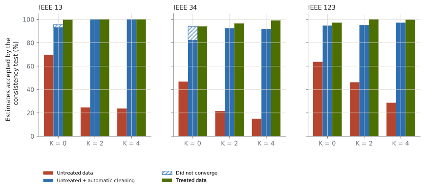
Without treatment, the estimator fails a large part of the time. Without sensors, only 70% (IEEE 13), 47% (IEEE 34) and 64% (IEEE 123) of the estimates are accepted. With sensors, acceptance drops to 15%–46%. This is not a fault of the sensors: with real measurements on the network, the estimator can now tell that the load data is wrong, instead of silently accommodating it.

Prior treatment solves consistency. With treated data, acceptance stays between 94% and 100% in all cases.

Automatic cleaning without sensors is misleading. It raises acceptance to 82%–95%, but on IEEE 13 and IEEE 34 the estimator fails to converge in 2.5% and 12% of cases: by de-weighting pseudo-measurements with no other source of information, parts of the network are left without enough observation. With 2 or 4 sensors, the non-convergence disappears.

4.2 Quality: how large the errors are

Figure 2 shows the median and the 10% to 90% range of voltage and per-bus load errors, across all estimates that converged, accepted or not.

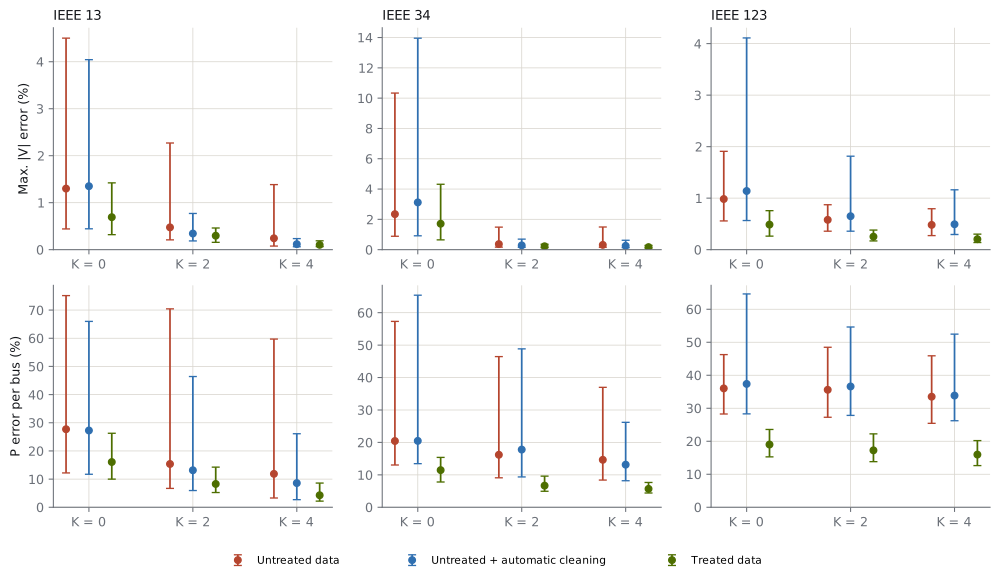
Feeder	Approach	Sensors	|V| error (median)	|V| error (worst 10%)	P error per bus
IEEE 13	Untreated	0	1.30%	4.50%	27.7%
	Treated	0	0.69%	1.42%	16.1%
	Untreated + cleaning	4	0.12%	0.24%	8.6%
	Treated	4	0.10%	0.19%	4.3%
IEEE 34	Untreated	0	2.34%	10.3%	20.4%
	Treated	0	1.71%	4.32%	11.5%
	Untreated + cleaning	4	0.25%	0.62%	13.1%
	Treated	4	0.17%	0.28%	5.7%
IEEE 123	Untreated	0	0.98%	1.91%	36.0%
	Treated	0	0.49%	0.76%	19.0%
	Untreated + cleaning	4	0.49%	1.16%	33.8%
	Treated	4	0.20%	0.30%	16.0%

Four conclusions follow from the table:

• Prior treatment reduces the median voltage error by 27% to 50% and the load error by 42% to 47%, with no new equipment.
• Sensors and treatment add up. With treated data, four sensors reduce the median voltage error from 0.69% to 0.10% on IEEE 13, from 1.71% to 0.17% on IEEE 34, and from 0.49% to 0.20% on IEEE 123. On IEEE 34, the worst tenth of the scenarios drops from 4.3% to 0.28%.
• With sensors, automatic cleaning comes close to prior treatment on the smaller feeders, where the sensors create enough local redundancy to point out which pseudo-measurement is wrong (IEEE 13: 0.12% versus 0.10%). On IEEE 123, with 85 load buses and only four sensors, this does not happen: the error stays at the level of untreated data. Automatic cleaning depends on measurement density.
• The load at each bus remains tied to the quality of customer data. Even with four sensors, the load error only falls below 6% where the data was treated and the network is small or medium-sized.

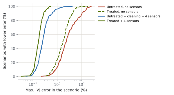
Figure 3 shows the full distribution of the voltage error on IEEE 34. Without treatment and without sensors, 38% of the scenarios have an error above 3%. With treated data and four sensors, none exceeds 0.6%.

5. Discussion and limitations

The study separates two things that usually get mixed up when "the estimator doesn't converge".

The first is the quality and standardization of the load data. Converting readings to the right instant, filling gaps with the typical profile, assigning each meter the uncertainty of its integration interval, and using the generation registry to resolve the flow direction of prosumers take the estimator from "unreliable most of the time" to "consistent almost always". This is data work, it can be automated, and it is the first thing to do.

The second is the lack of measurement on the network itself. Without it, the estimator cannot distinguish wrong load data from an unusual network state, and automatic cleaning can even make the result worse. A few well-placed synchronized sensors provide that reference: they confirm or contradict the pseudo-measurements, reduce the voltage error by an order of magnitude on long feeders, and make automatic cleaning viable where measurement density is sufficient.

Limitations:

• Synthetic defects. The rates of coverage, missing data, gross errors and generation were chosen to represent typical problems, not measured on a real network; the absolute numbers depend on them, and the ranking between strategies is the most robust result.
• A snapshot in time. Time series were not used; they would allow better treatments (interpolation by consumption pattern, Kalman filters) and detection of persistent defects.
• Known taps and correct topology. Topology and phase-assignment errors in the network records, common in practice, were left for a separate study.
• Numerical convergence. Gauss-Newton in rectangular coordinates, starting from no-load voltages, converged in almost all cases; failure showed up mostly as inconsistency. Commercial implementations may use different criteria and formulations, but the mechanism, inconsistent data with little redundancy, is the same.

6. Conclusion

On three test feeders with distributed generation and load data with realistic defects, untreated data caused the estimator to be rejected by the consistency test in 30% to 53% of the scenarios. Prior data treatment reduced rejection to 0.5%–6% and the median voltage error by 27% to 50%. Automatic residual-based cleaning, without network measurements, masked the problem and caused convergence failures. With two to four synchronized sensors, automatic cleaning started to work on the smaller feeders, and the combination of treated data and four sensors brought the median voltage error down to 0.10%–0.20%. For ADMS operators, the message is twofold: treating load data is the condition for the estimator to converge, and measuring at a few points on the network is what makes the result trustworthy and allows the cleaning to be automated.

Reproducibility

Code: senl.py (nonlinear estimator, automatic cleaning), study2.py (defects, treatments and scenarios) and figs2.py. It uses the network model from the previous note, se3f.py. Results: IEEE 13, IEEE 34, IEEE 123. Dependencies: Python 3.12 or later, OpenDSSDirect.py, NumPy, SciPy and Matplotlib. Seed: 2026.

References

1. M. E. Baran and A. W. Kelley, "State estimation for real-time monitoring of distribution systems," IEEE Transactions on Power Systems, vol. 9, no. 3, 1994.
2. A. Primadianto and C.-N. Lu, "A review on distribution system state estimation," IEEE Transactions on Power Systems, 2017.
3. G4W, "How many sensors, and where? Synchronized measurement placement for three-phase state estimation in distribution feeders," Technical note G4W-NT-2026-01, 2026. Available at: /en/insights/alocacao-sensores-observabilidade/
4. A. Abur and A. Gómez Expósito, Power System State Estimation: Theory and Implementation. New York: Marcel Dekker, 2004.
5. A. Monticelli, State Estimation in Electric Power Systems: A Generalized Approach. Boston: Kluwer Academic Publishers, 1999.
6. W. H. Kersting, "Radial distribution test feeders," in Proc. IEEE PES Winter Meeting, 2001.
7. EPRI, OpenDSS — Open Distribution System Simulator. Available at: https://sourceforge.net/projects/electricdss/
8. DSS-Extensions, OpenDSSDirect.py and electricdss-tst (OpenDSS test cases). Available at: https://github.com/dss-extensions